How I recreated this timelapse of the MESSENGER flyby of Earth
In 2005, NASA’s MESSENGER spacecraft flew by Earth on its way to Mercury and as it departed, turned back to take 1080 photos of Earth over a period of 24 hours. In that time it flew 370,287 km just beyond the orbit of the Moon.
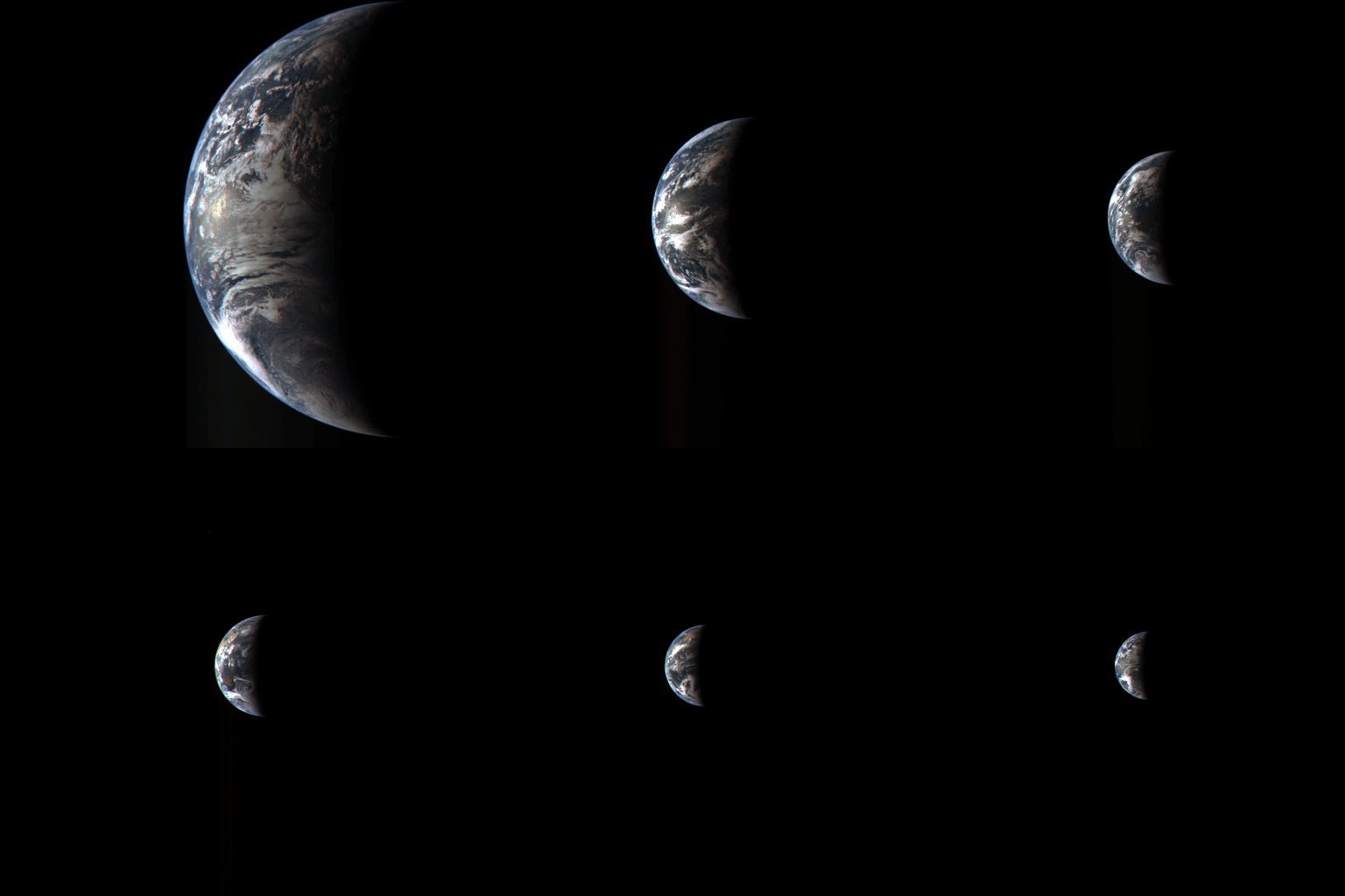
Unfortunately, back in 2005, video compression technology was not particularly advanced and so when NASA released this timelapse, it was significantly lower in quality. (Right click and click Play if the video doesn’t autoplay)
Pulling the archive image data
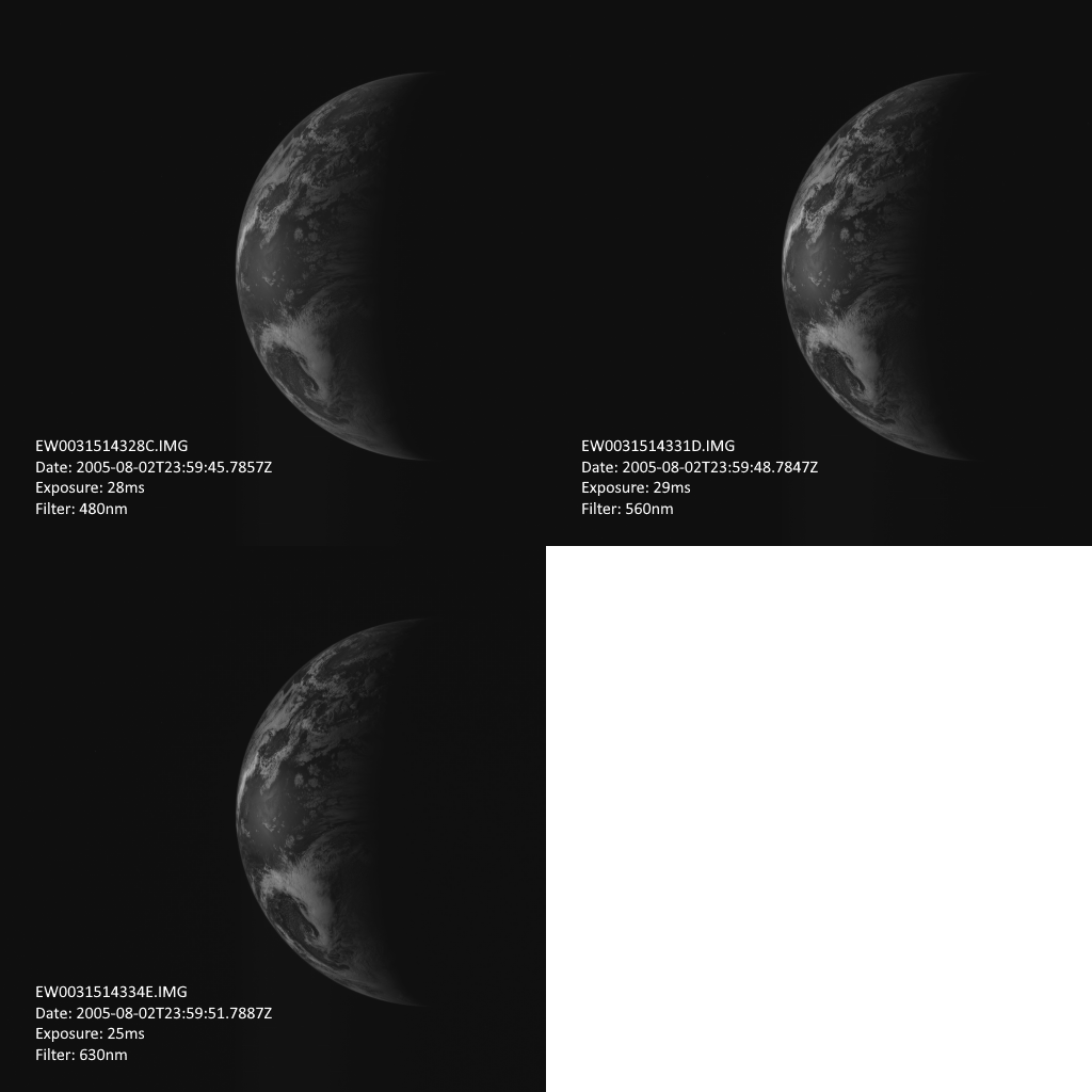
NASA makes most of its images publicly available via their Planetary Data System or PDS. After a bit of digging I found the image data from MESSENGER for this time period in this directory. Each image is stored in two files an IMG image and an XML metadata file. The IMG format is NASA’s uncompressed 16bit image format. The XML file contains additional metadata such as exposure time, ship position and attitude as well as filter information. In fact each frame of this timelapse consists of 3 separate images taken through different red, green and blue filters.
Transforming the images
After downloading all the required images from the PDS archive, I had to convert them into a format that I could work with. There are a few tools that allow you to manually open and manipulate IMG files such as NasaView or QGIS. Initially, I used GDAL an open source command line tool for transforming and working with all kinds of geospatial data formats. To convert the 1080 IMG files to 16bit TIFF, I wrote a script to run the following command:
gdal_translate.exe -of GTiff -ot UInt16 -scale 0 4095 0 65535 <input>.xml <output>.tif
The scale parameter adjusts the input value range from 0-4095 to 0-65535
Then to combine the red, green and blue images into a single frame, I used python’s CV2 library:
def combine(image1, image2, image3, output_image):
    img1 = cv2.imread(image1, cv2.IMREAD_GRAYSCALE)
    img2 = cv2.imread(image2, cv2.IMREAD_GRAYSCALE)
    img3 = cv2.imread(image3, cv2.IMREAD_GRAYSCALE)

    rgb_image = cv2.merge((img1, img2, img3))
    cv2.imwrite(output_image, rgb_image)
I then used ffmpeg to convert these into a gif:
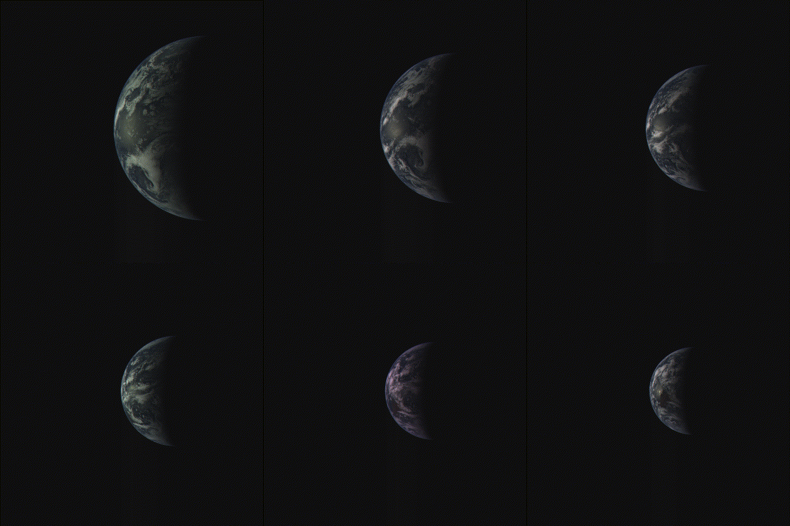
However, the resulting images have wildly incorrect exposure and colour. This is because each image was taken with a different shutter speed including the individual red, green and blue images of the same frame. In this frame for example, its blue component is clearly overly represented.
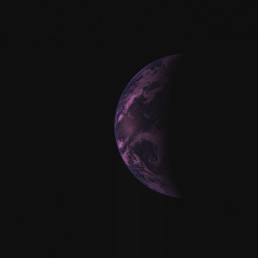
This can be confirmed by looking at the metadata of each image:
Red (EW0031519848C.xml):
<start_date_time>2005-08-03T01:31:45.7857Z</start_date_time>
<img:exposure_duration unit="ms">28</img:exposure_duration><!-- EXPOSURE_DURATION -->
<img:exposure_type>Auto</img:exposure_type><!-- EXPOSURE_TYPE -->
Green (EW0031519851D.xml):
<start_date_time>2005-08-03T01:31:48.7987Z</start_date_time>
<img:exposure_duration unit="ms">15</img:exposure_duration><!-- EXPOSURE_DURATION -->
<img:exposure_type>Auto</img:exposure_type><!-- EXPOSURE_TYPE -->
Blue (EW0031519854E.xml):
<start_date_time>2005-08-03T01:31:51.7877Z</start_date_time>
<img:exposure_duration unit="ms">26</img:exposure_duration><!-- EXPOSURE_DURATION -->
<img:exposure_type>Auto</img:exposure_type><!-- EXPOSURE_TYPE -->
We can see that due to the auto exposure, the green channel was only exposed for half the time of the other two channels resulting in an overly blue image.
Normalising for exposure time
To compensate for the different exposure times, I tried to adjust the brightness of each photo to match a target exposure time of 40 ms using the following code:
def adjust_exposure(image, actual_exposure_time, target_exposure_time):
    exposure_ratio = target_exposure_time / actual_exposure_time
    return cv2.convertScaleAbs(image, alpha=exposure_ratio, beta=0)
This seemed to fix the exposure of the Earth but incorrectly adjusted the colour of the dark background pixels resulting in even more flickering:
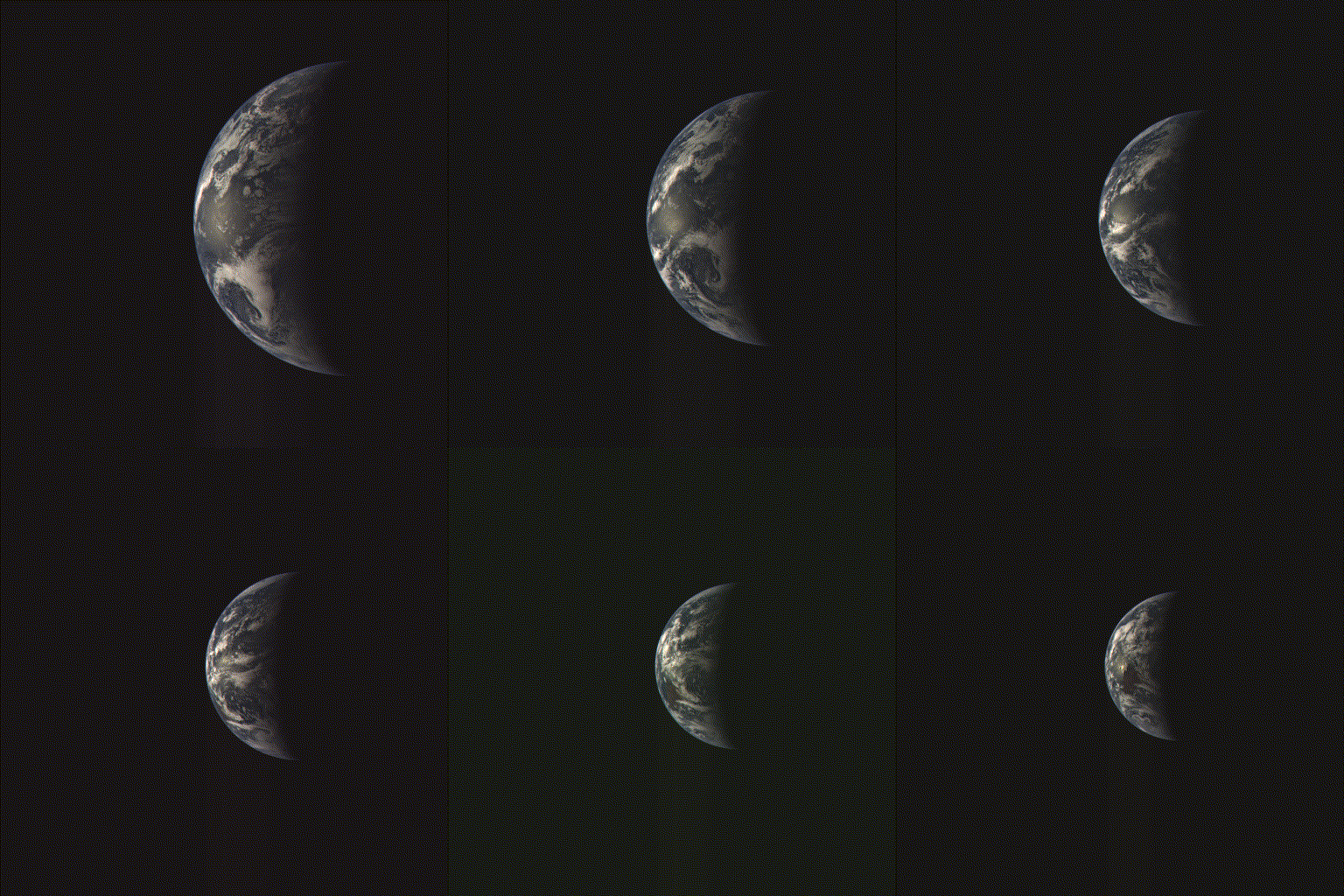
Here is that same frame as before after boosting its green channel. As you can see the background is now the wrong colour.
Taking a step back
Clearly, correcting the raw satellite image data is going to be a bit more complicated than I had first hoped. However, I noticed a file called CALINFO.TXT alongside the image data on the PDS Imaging Node Server. It states:
The CALIB directory contains files needed to reduce raw MDIS images (EDRs)
to units of radiance or I/F. Files needed for major corrections are
arranged into subdirectories by correction type.
This could be promising. Radiance is a measure of the amount of light being reflected from a surface. This is what we really need to display in our final images. The TXT file continues:
Raw units are of DN converted to the physical units
of radiance or I/F, following the calibration equation:

L(x,y,f,T,t,b) = Lin[DN(x,y,f,T,t,b) - Dk(x,y,T,t,b) -
Sm(x,y,t,b)] / {Flat(x,y,f,b) * t * Resp(f,b,T)}
DN simply means Digital Number i.e. the raw pixel data of the original images. To calculate the radiance value, we just need to pass the raw values through a series of functions. It continues to describe each function:
L(x,y,f,T,t,b) is radiance in units of W / (m**-2 microns**-1 sr**-1),
measured by the pixel in column x, row y, through filter f, at CCD
temperature T and exposure time t, for binning mode b,

DN(x,y,f,T,t,T) is the raw DN measured by the pixel in column x, row
y, through filter f, at CCD temperature T and exposure time t, for binning
mode b,

Dk(x,y,T,t,b) is the dark level in a given pixel, derived from
a model based on exposure time and CCD temperature,

Sm(x,y,t,b) is the scene-dependent frame transfer smear for the pixel,

Lin is a function that corrects small nonlinearity of detector response,

Flat(x,y,f,b) is the non-uniformity or 'flat-field' correction,

Resp(f,b,T) is the responsivity, relating dark-, flat-, and
smear-corrected DN per unit exposure time to radiance,

and

t is the exposure time.
Feeling slightly daunted, I began the task of implementing these calibration functions in python. The documentation
appears to provide most of the necessary information and I was able to implement the Dk (dark level) function.
def dark_polynomial(variable, darktable, T):
    # C(T) = H0 + H1 * T + H2 * T**2 + H3 * T**3
    return (darktable[variable][0] +
            darktable[variable][1] * T +
            darktable[variable][2] * math.pow(T, 2) +
            darktable[variable][3] * math.pow(T, 3))


def calibrate_dark(pds_image, darktable):
    T = pds_image.label['MESS:CCD_TEMP']
    C = dark_polynomial('C', darktable, T)
    D = dark_polynomial('D', darktable, T)
    E = dark_polynomial('E', darktable, T)
    F = dark_polynomial('F', darktable, T)
    O = dark_polynomial('O', darktable, T)
    P = dark_polynomial('P', darktable, T)
    Q = dark_polynomial('Q', darktable, T)
    S = dark_polynomial('S', darktable, T)

    t = pds_image.label['MESS:EXPOSURE']

    img = pds_image.image

    for y in range(img.shape[1]):
        for x in range(img.shape[0]):
            dn = img[y, x]
            dk = C + D + (E + F * t) * y + (O + P * t + (Q + S * t) * y) * x
            if dk < dn:
                img[y, x] = dn - dk
            else:
                img[y, x] = 0
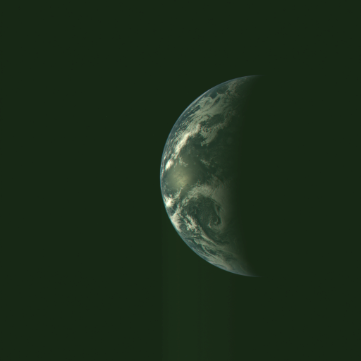
With the dark level calibrated and the same exposure adjustment as before, we get the following result: